
Optional features are specialized modules that can be added to UDEC at an additional cost. For more information or to purchase, please click here.
Fluid Flow in Joints in UDEC
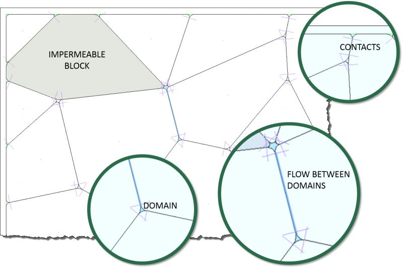
UDEC has the capability to perform the analysis of fluid flow through the fractures and voids of a system of impermeable blocks. Steady-state pore pressures can be assigned to zones within deformable blocks and boundary conditions may be applied in terms of fluid pressures or by defining an impervious boundary. A porous medium can be defined around the UDEC block model to simulate a regional flow field.
The numerical implementation for fluid flow in UDEC makes use of the domain structure. For a closely packed system, there is a network of domains, each of which is assumed to be filled with fluid at uniform pressure and which communicates with its neighbors through contacts. Domains are separated by the contact points, which are the points at which the forces of mechanical interaction between blocks are applied. Because deformable blocks are discretized into a mesh of triangular elements, gridpoints may exist not only at the vertices of the block, but also along the edges. A contact point will be placed wherever a gridpoint meets an edge or a gridpoint of another block. Therefore, the degree of refinement of the numerical representation of the flow network is linked to the mechanical discretization adopted. In the absence of gravity, a uniform fluid pressure is assumed to exist within each domain. For problems with gravity, the pressure is assumed to vary linearly according to the hydrostatic gradient, and the domain pressure is defined as the value at the center of the domain. Flow is governed by the pressure differential between adjacent domains.
The fluid-flow calculation can also be run either coupled or uncoupled with the mechanical stress calculation. A fully coupled mechanical-hydraulic analysis is performed in which fracture conductivity is dependent on deformation, and conversely, joint fluid pressures affect the mechanical computations. Both confined flow and flow with a free surface can be modeled with this formulation. Flow is idealized as laminar viscous flow between parallel plates. A visco-plastic flow model is also available to simulate flow of cement grout in the joints. The joint permeability relation can be modified and one-way thermal-hydraulic coupling of flow in joints, in which temperature variations induce changes in the viscosity and density of water, can also be simulated.
The fluid-calculation modes available include the following.
- Compressible Liquid, Steady-State Flow
- Compressible Liquid, Transient Flow
- Incompressible Liquid, Transient Flow
- Compressible Gas, Transient Flow
- Two-Phase Fluid, Transient Flow
Barton-Bandis Joint Model
The Barton-Bandis joint model utilizes a series of empirical relations for joint normal behavior and joint shear behavior based on the effects of surface roughness on discontinuity deformation and strength as described by Barton (1982) and Bandis et al. (1985). The Barton-Bandis joint model encompasses the following features.
Joint Shear Behavior
- Dilation as function of normal stress and shear displacement.
- Joint damage due to post-peak shear.
- Reduced secondary peak shear upon post-peak shear reversal.
Joint Normal Behavior
- Hyperbolic stress-displacement path.
- Hysteresis due to successive load/unload cycles.
- Normal stiffness increase due to successive load/unload cycles.
- Normal stiffness change due to surface mismatch caused by shear displacement.
- Hydraulic aperture calculation based on joint closure and joint roughness.
Thermal Analysis
The thermal model simulates the transient flux of heat in materials and the subsequent development of thermally induced stresses. The heat flux is modeled by either isotropic or anisotropic conduction. Heat sources can be added and can be made to decay exponentially with time.
UDEC allows simulation of transient heat conduction in materials and the development of thermally induced displacements and stresses. This includes the following specific features.
- Heat transfer is modeled as conduction, either isotropic or anisotropic, depending on the user’s choice of material properties.
- Several different thermal boundary conditions may be imposed.
- Any of the mechanical block models may be used with the thermal model.
- Heat sources may be inserted into the material as volume sources. The sources may be made to decay exponentially with time.
- Both implicit and explicit calculations schemes are available, and the user can switch from one to the other at any time during a run.
- The thermal analysis provides one-way coupling to the mechanical stress calculation through the thermal expansion coefficient.
- The thermal analysis provides one-way coupling to the calculation for fluid flow in joints through the temperature dependency of fluid density and joint permeability.
Example
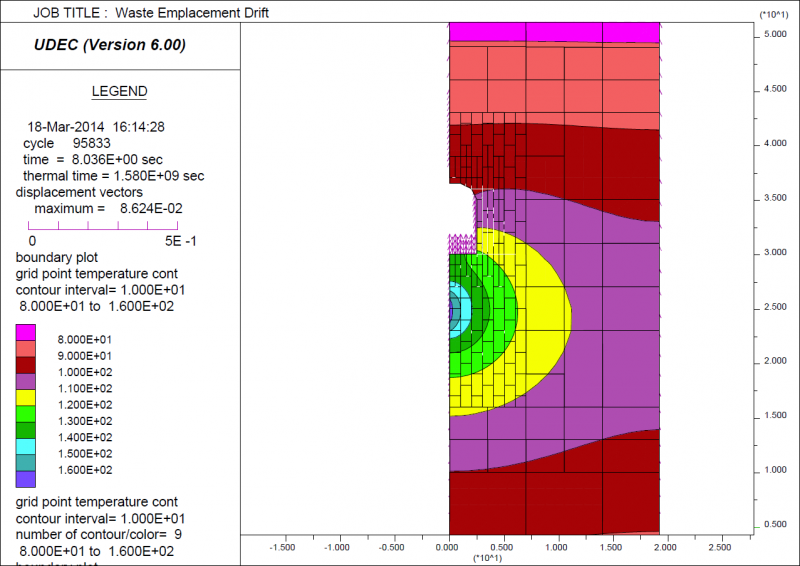
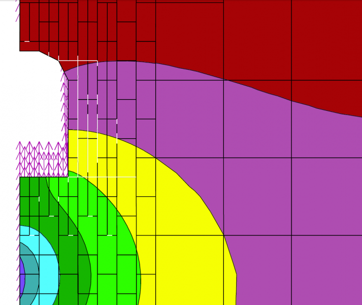
The following example shows a transient thermal-mechanical simulation of the behavior of a nuclear-waste emplacement drift in which heat-producing waste is placed vertically beneath the panel floor (Christianson, 1989). The emplacement drift under study is in the center of an emplacement panel. Waste canisters are placed in the floor of the drift. Using model symmetry, only one-half of the disposal room-and-pillar needs to be included in the analysis. The thermal boundary conditions are considered to be adiabatic.
The tributary heating area for the emplacement panel is reported to be 8194.5 m2. The average thermal loading is considered to be 14.1 W/m2. For the panel geometry, this results in an initial heat-generating power per meter of room length of 713.5 W. The initial power of a waste container at the time of emplacement varies from 0.42 kW to 3.2 kW. The following UDEC model shows the rock mass around the panel with the temperate distribution and thermal-induced rock displacements after 50 years since waste emplacement.
Creep Material Models
The creep option can be used to simulate the behavior of materials that exhibit creep (i.e., time-dependent material behavior). The major difference between creep and other constitutive models is the concept of problem time in the simulation. For creep runs, the problem time and timestep represent real time, while for static analysis (in the other constitutive models), the timestep is an artificial quantity used only as a means of stepping to a steady-state condition. The timestep may be set by the user to a constant value, or controlled by UDEC to change automatically. If the timestep is changed automatically, it can be decreased whenever the maximum unbalanced force exceeds some threshold, and increased whenever it goes below some other level. For some of the creep models available, the creep rate is temperature dependent. Temperatures may be either specified as a model property or calculated during cycling using the thermal mode of the code. For either case, a temperature gradient also may be specified.
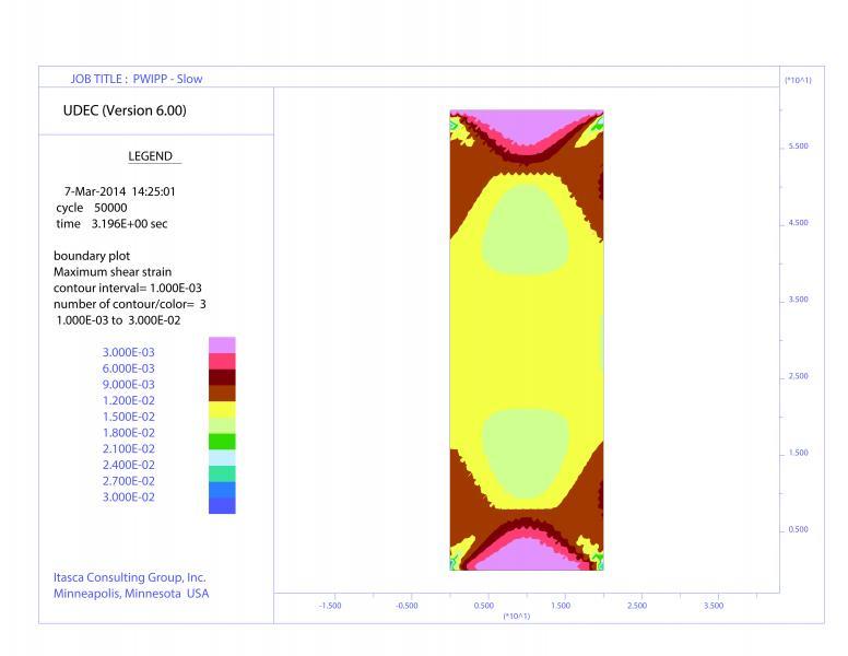
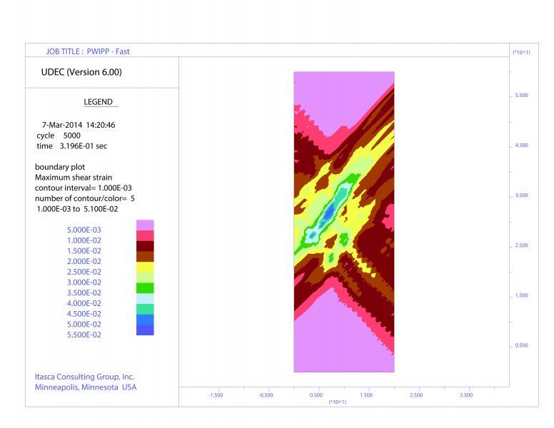
Unconfined compression tests are performed with a creep model as a demonstration simulating localization given an appropriate loading rate. Under a low strain rate (top) the response is monotonic with the sample deforming uniformly over 139 hours. However, given a 10x faster strain rate (bottom), shear bands are predicted to form. Although the maximum load is nearly the same for the two tests, the latter one exhibits global softening behavior.
Eight creep models have been implemented in UDEC as described below in order of increasing complexity.
Classical Viscoelastic (Maxwell) Model
Viscoelastic materials exhibit both viscous and elastic behaviors. The classical notion of Newtonian viscosity is that the rate of strain is proportional to stress. Stress-strain relations can be developed for viscous flow in a way similar to the way relationships are developed for elastic deformation.
Burgers Viscoelastic Model
The Burgers model is composed of a Kelvin model and a Maxwell model connected in series.
Two-Component Power Law
The Norton power law (Norton, 1929) is commonly used to model the creep behavior of salt or potash. The standard form of this law calculates the creep rate as a function of two material constants (A and n) and deviatoric stress:
WIPP Model
The WIPP (Waste Isolation Pilot Plant) model is a reference (empirical) viscoelastic creep law commonly used in thermomechanical analyzes associated with studies of underground nuclear-waste isolation in salt. This model describes the time- and temperature-dependent creep of natural rock salt.
Burgers Viscoplastic Model
The Burgers-creep viscoplastic model in UDEC is characterized by a visco-elasto-plastic deviatoric behavior and an elasto-plastic volumetric behavior. The viscoelastic and viscoplastic strain-rate components are assumed to act in series. The viscoelastic constitutive law corresponds to a Burgers model (Kelvin cell in series with a Maxwell component), and the plastic constitutive law corresponds to a Mohr-Coulomb model.
Power Law Viscoplastic Model
The viscoplastic model combines the behavior of the viscoelastic two-component Norton power law and the Mohr-Coulomb elastoplastic models.
WIPP Viscoplastic Model
Viscoplasticity is also modeled by combining the viscoelastic WIPP model with the Drucker-Prager plasticity model. Of the plasticity models currently available in UDEC, the Drucker-Prager model is the most compatible with the WIPP-reference creep law, because both models are formulated in terms of the second invariant of the deviatoric stress tensor.
Crushed Salt Model
The crushed-salt constitutive model is implemented in UDEC to simulate volumetric and deviatoric creep compaction behaviors. The model is a variation of the WIPP-reference creep law and is based on the model described by Sjaardema and Krieg (1987) with an added deviatoric component as proposed by Callahan and DeVries (1991).
User-Defined Models (UDM)
With this option, users may create their own contact or zone constitutive model for use in UDEC. The model must be written in C++ (CPP) and compiled as a DLL (dynamic link library) file using Microsoft Visual Studio 2010. The DLL then can be loaded whenever it is needed. The main function of the zone model is to return new stresses, given strain increments. The main function of the contact constitutive model is to return forces given displacements. However, the model must also provide other information (such as name of the model and material property names) and describe certain additional details about how the model interacts with the code. It is assumed that the user has a working knowledge of the C++ programming language.
UDMs may be used in other Itasca software provided this option is also available for that software. New DLL models can be obtained from an Itasca website devoted specifically to model development and exchange: User-Defined Constitutive Models (UDM).
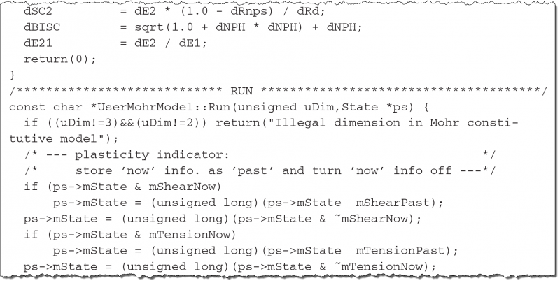
Instructions for writing a constitutive model in C++ for operation in UDEC and the implementation of a DLL model are provided, including:
- Descriptions of the base class and member functions;
- Registration of models;
- Information passed between the model and UDEC;
- The model state indicators;
- Descriptions of the support functions used by the model;
- The source code for an example model;
- FISH support for user-written models;
- The mechanism for creating and loading a DLL; and
- Microsoft Visual Studio 2010 constitutive model templates are also provided to assist in creating new constitutive models.